R Modes Package.
Note: Please Download from CRAN repository; the links to the left are unstable. The CRAN package for using the modes package in R is: https://cran.r-project.org/web/packages/modes/index.html and the tarball itself is available from https://cran.r-project.org/src/contrib/modes_0.6.1.tar.gz
Sorry about the mess! I'm still learning how to use Github/Git.
Description
Tutorial
12 Examples of the most useful and common features of this package are included below.
Nonparametric Examples
1. Mode examples
Example 1.1
data<-c(rep(6,9),rep(3,3))
mode(data,type=1,"NULL","NULL")
       [,1]
Value     6
Length    9
Example 1.2
set.seed(1246)
data<-c(rep(6,9),rep(3,9))
mode(data,type=1,"NULL","NULL")
       [,1] [,2]
Value     3    6
Length    9    9
Example 1.3
set.seed(1246)
data<-c(rep(6,9),rep(3,8),rep(7,7),rep(2,6))
mode(data,type=1,"NULL",2)
       [,1] [,2] [,3] [,4]
Value     6    3    7    2
Length    9    8    7    6
Example 1.4
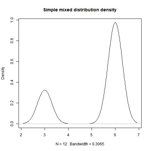
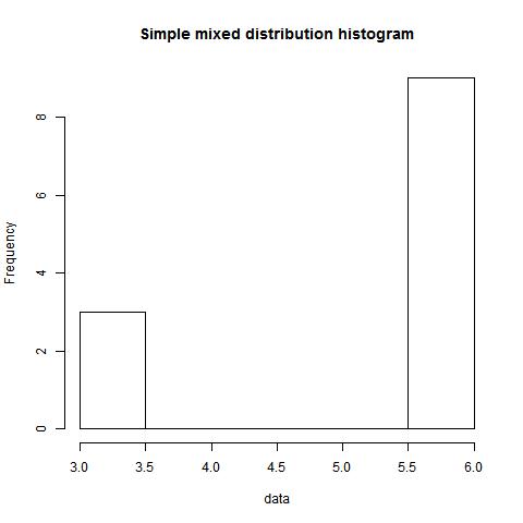
set.seed(1246)
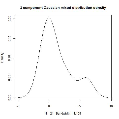
data<-c(rnorm(15,0,1),rnorm(21,5,1),rep(3,3))
modes(data)
       [,1]
Value     0
Length   12
Example 1.5
    set.seed(1246)
    data<-c(rep(6,3),rep(3,3),rnorm(15,0,1))
    modes(data,3,NULL,4)
    modes(data,type=2,digits=1,3)
       [,1] [,2] [,3]                   [,4]
Value  "3"  "6"  "-0.00528877744563036" "-0.265047873213653"
Length "3"  "3"  "1"                    "1"
       [,5]                 [,6]                 [,7]
Value  "-0.383946266260758" "-0.503595358662098" "-0.890103993657086"
Length "1"                  "1"                  "1"
       [,8]                 [,9]                 [,10]
Value  "-0.902559181415477" "-0.929018190441427" "-1.51710239243673"
Length "1"                  "1"                  "1"
       [,11]               [,12]               [,13]
Value  "0.196147751721519" "0.216425886134856" "0.400936002681914"
Length "1"                 "1"                 "1"
       [,14]               [,15]               [,16]
Value  "0.461525542956227" "0.541086638435628" "1.3029586964899"
Length "1"                 "1"                 "1"
       [,17]
Value  "1.34537915481889"
Length "1"
Warning message:
In modes(data, 3, NULL, 4) : A single observation
         is being observed as a mode.
        Double check the class or inspect the data.
        Alternatively, you may have specified 'nmore' too many times
        for this data.
modes(data,type=2,digits=1,3)
        [,1] [,2] [,3] [,4] [,5] [,6] [,7] [,8]
Value  -0.9    3    6   -2 -0.5 -0.3  0.2  0.5
Length  3.0    3    3    1  1.0  1.0  2.0  2.0
Warning message:
In modes(data, type = 2, digits = 1, 3) : A single observation
         is being observed as a mode.
        Double check the class or inspect the data.
        Alternatively, you may have specified 'nmore' too many times
        for this data.
2) Other General Parametric Examples
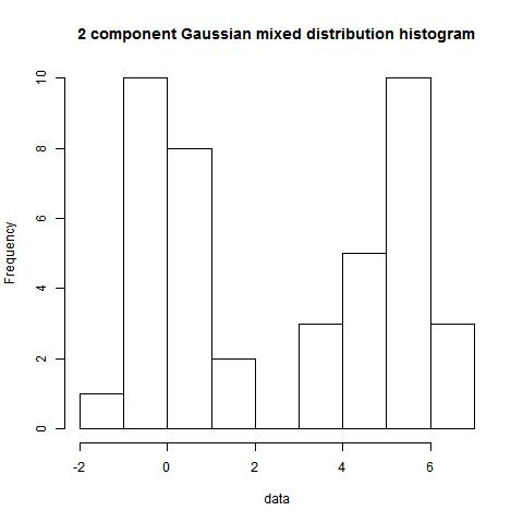
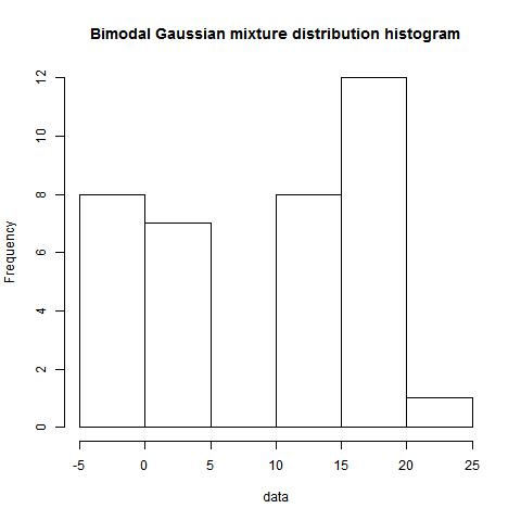
Example 2.1
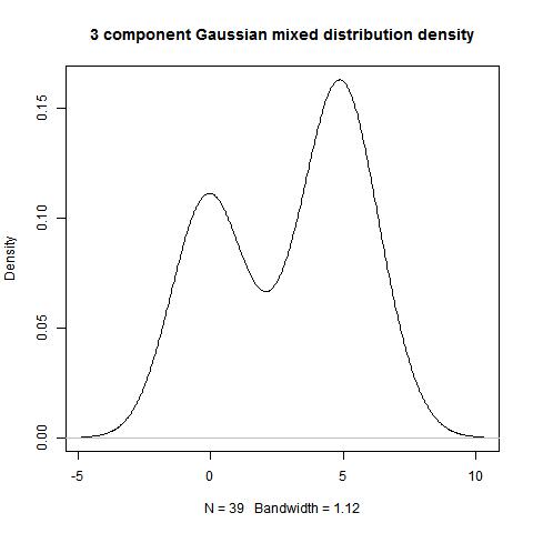
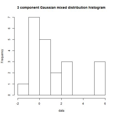
set.seed(1246)
data<-c(rnorm(15,0,1),rnorm(21,5,1))
hist(data)
bimodality_amplitude(data,TRUE)
bimodality_coefficient(data,TRUE)
bimodality_ratio(data,FALSE)

> bimodality_amplitude(data,TRUE)
[1] 0.5343913
> bimodality_coefficient(data,TRUE)
[1] 0.8894365
> bimodality_ratio(data,FALSE)
Amplitude (y)
     1.413765
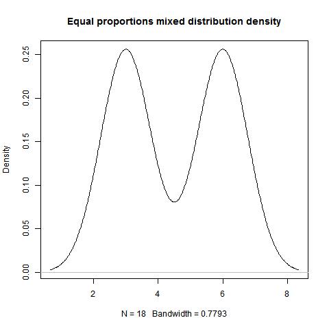
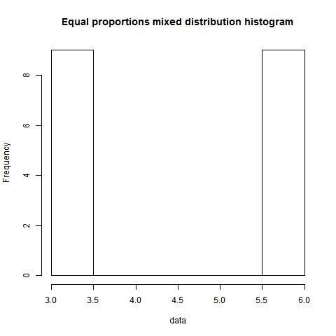
Example 2.2
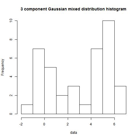
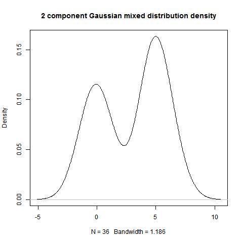
set.seed(1246)
data<-c(rnorm(21,0,1),rnorm(21,5,1))
hist(data)
bimodality_amplitude(data,TRUE)
bimodality_coefficient(data,TRUE)
bimodality_ratio(data,FALSE)
> bimodality_amplitude(data,TRUE)
[1] 0.5569044
> bimodality_coefficient(data,TRUE)
[1] 0.880667
> bimodality_ratio(data,FALSE)
Amplitude (y)
    0.9039876
3) Mixture Proportions Examples
Example 3.1
set.seed(1246)
dist1<-rnorm(21,5,2)
dist2<-dist1+11
data<-c(dist1,dist2)
hist(data)
bimodality_amplitude(data,TRUE)
bimodality_ratio(data,FALSE)
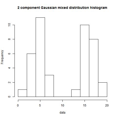
> bimodality_amplitude(data,TRUE)
[1] 0.6894354
> bimodality_ratio(data,FALSE)
Amplitude (y)
     1.000229
Example 3.2
set.seed(1246)
dist1<-rnorm(21,-15,1)
dist2<-rep(dist1,3)+30
data<-c(dist1,dist2)
hist(data)
bimodality_amplitude(data,TRUE)
bimodality_ratio(data,FALSE)
> bimodality_amplitude(data,TRUE)
[1] 1
> bimodality_ratio(data,FALSE)
Amplitude (y)
     2.999414
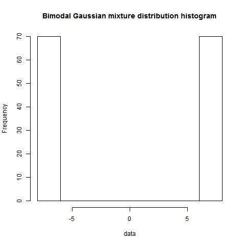
Example 3.4
dist1<-rep(7,70)
dist2<-rep(-7,70)
data<-c(dist1,dist2)
hist(data)
bimodality_ratio(data,FALSE)
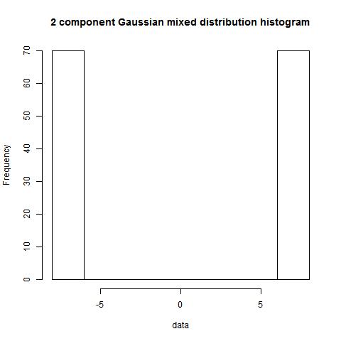
> bimodality_ratio(data,FALSE)
Amplitude (y)
            1
Parametric Examples
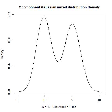
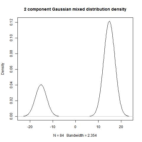
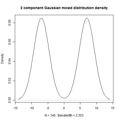
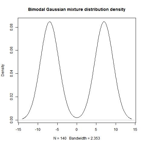
4) Replicating a two component Gaussian (normal) mixture
Example 4.1
Draw data & plot the distribution
set.seed(1246)
dist1<-rnorm(14,-5,1)
dist2<-rnorm(21,5,1)
plot(density(c(dist1,dist2)), main="Bimodal Gaussian mixture distribution")
Calculate the means and standard deviations
mu1<-mean(dist1)
mu2<-mean(dist2)
sd1<-sd(dist1)
sd2<-sd(dist2)
Apply measures
Ashmans_D(mu1,mu2,sd1,sd2)
bimodality_separation(mu1,mu2,sd1,sd2)
> Ashmans_D(mu1,mu2,sd1,sd2)
[1] 12.10559
> bimodality_separation(mu1,mu2,sd1,sd2)
[1] -3.061472
>
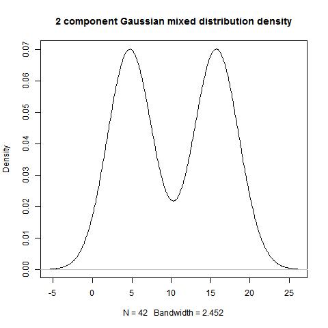
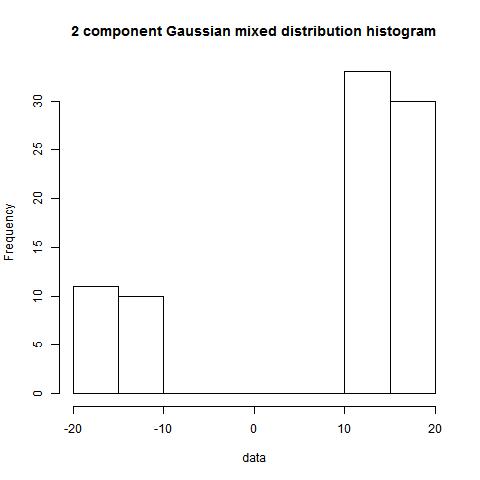
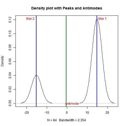
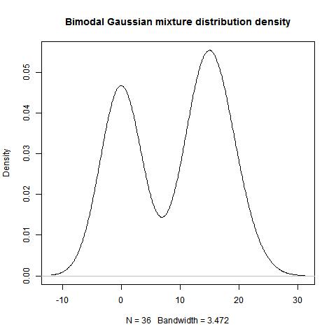
5) Applying to know mixture components
Example 5.1
Draw data & plot the distribution
set.seed(1246)
data<-c(rnorm(15,0,1),rnorm(21,15,3))
plot(density(c(dist1,dist2)), main="Bimodal Gaussian mixture distribution")
Apply measures
Ashmans_D(mu1,mu2,sd1,sd2)
bimodality_separation(mu1,mu2,sd1,sd2)
> Ashmans_D(mu1,mu2,sd1,sd2)
[1] 12.10559
> bimodality_separation(mu1,mu2,sd1,sd2)
[1] -3.061472
References
Ashman, K., Bird, C., & Zepf, S. (1994). Detecting bimodality in astronomical datasets. The Astronomical Journal, 2348-2361.
Ellison, A. (1987). Effect of Seed Dimorphism on the Density-Dependent Dynamics of Experimental Populations of Atriplex triangularis (Chenopodiaceae). American Journal of Botany, 74(8), 1280-1288.
Zhang, C., Mapes, B., & Soden, B. (2003). Bimodality in tropical water vapour. Quarterly Journal of the Royal Meteorological Society, 129(594), 2847-2866.
Designer Templates
We’ve crafted some handsome templates for you to use. Go ahead and click 'Continue to layouts' to browse through them. You can easily go back to edit your page before publishing. After publishing your page, you can revisit the page generator and switch to another theme. Your Page content will be preserved.
Authors and Contributors
You can @mention a GitHub username to generate a link to their profile. The resulting <a> element will link to the contributor’s GitHub Profile. For example: In 2007, Chris Wanstrath (@defunkt), PJ Hyett (@pjhyett), and Tom Preston-Werner (@mojombo) founded GitHub.